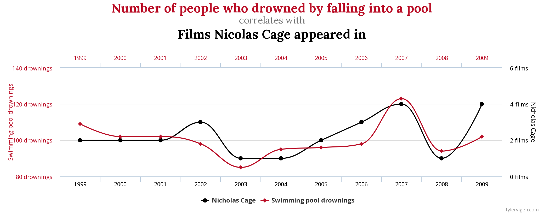
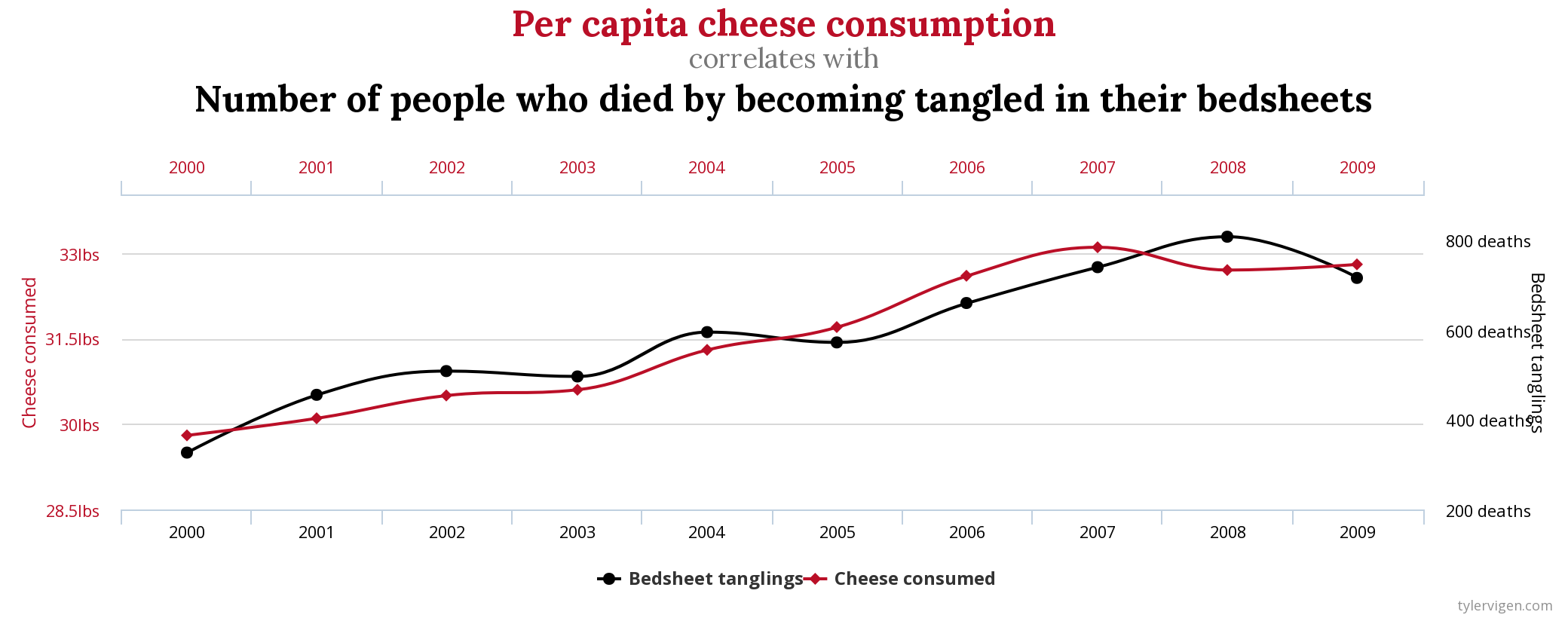
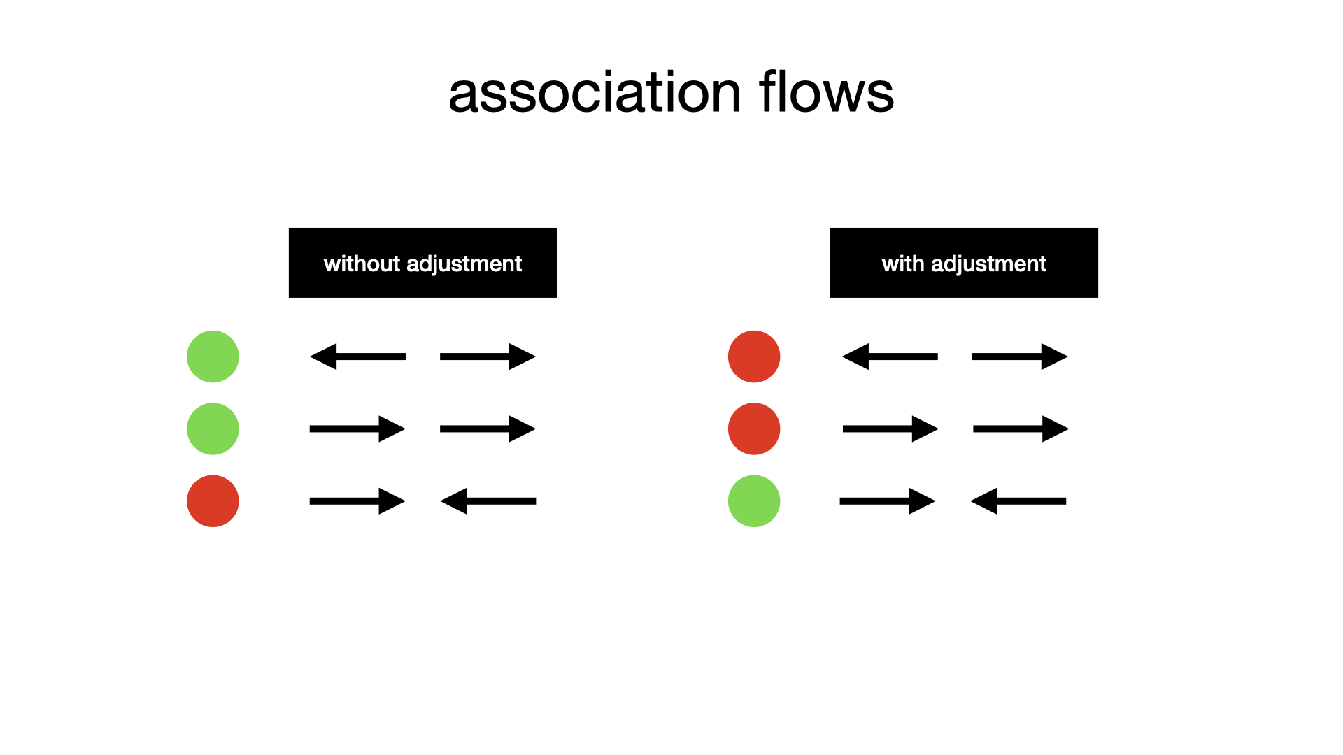
class: center middle main-title section-title-1 # Causal Diagrams .class-info[ **Session 7** .light[STA 379/679: Causal Inference <br> Lucy D'Agostino McGowan ] ] --- class: center <img src="img/twitter-correlation.png" height = "600"></img> --- class: title title-1 # What causes spurious correlations? 1. Random chance --- class: title title-1 # What causes spurious correlations? 1. Random chance 1. Confounders --- class: title title-1 # How do we correct for these? .pull-left[ .box-inv-1[Random chance] ] --- class: title title-1 # How do we correct for these? .pull-left[ .box-inv-1[Random chance] .box-1[Classic statistics!] ] --- class: title title-1 # How do we correct for these? .pull-left[ .box-inv-1[Random chance] .box-1[Classic statistics!] .box-1[Measures of uncertainty (i.e.confidence intervals)] ] ---  .footer[https://www.tylervigen.com/spurious-correlations] ---  --- .small[ ```r d <- tibble( year = 1999:2009, nic_cage = c(2, 2, 2, 3, 1, 1, 2, 3, 4, 1, 4), drownings = c(109, 102, 102, 98, 85, 95, 96, 98, 123, 94, 102), ) cor.test(~ nic_cage + drownings, data = d) ``` ``` ## ## Pearson's product-moment correlation ## ## data: nic_cage and drownings ## t = 2.6785, df = 9, p-value = 0.02527 ## alternative hypothesis: true correlation is not equal to 0 ## 95 percent confidence interval: ## 0.1101273 0.9045101 ## sample estimates: ## cor ## 0.6660043 ``` ] --- .small[ ```r d <- tibble( year = 1999:2009, nic_cage = c(2, 2, 2, 3, 1, 1, 2, 3, 4, 1, 4), drownings = c(109, 102, 102, 98, 85, 95, 96, 98, 123, 94, 102), ) cor.test(~ nic_cage + drownings, data = d) ``` ``` ## ## Pearson's product-moment correlation ## ## data: nic_cage and drownings ## t = 2.6785, df = 9, p-value = 0.02527 ## alternative hypothesis: true correlation is not equal to 0 ## 95 percent confidence interval: *## 0.1101273 0.9045101 ## sample estimates: ## cor ## 0.6660043 ``` ] --- class: title title-1 # How do we correct for these? .pull-left[ .box-inv-1[Random chance] .box-1[Classic statistics!] .box-1[Measures of uncertainty (i.e.confidence intervals)] ] .pull-right[ .box-inv-1[Confounders] ] --- class: title title-1 # How do we correct for these? .pull-left[ .box-inv-1[Random chance] .box-1[Classic statistics!] .box-1[Measures of uncertainty (i.e.confidence intervals)] ] .pull-right[ .box-inv-1[Confounders] .box-1[adjust for confounders!] ] ---  --- .small[ ```r d <- tibble( year = 2000:2009, bedsheets = c(327, 456, 509, 497, 596, 573, 661, 741, 809, 717), cheese = c(29.8, 30.1, 30.5, 30.6, 31.3, 31.7, 32.6, 33.1, 32.7, 32.8), ) cor.test(~bedsheets + cheese, data = d) ``` ``` ## ## Pearson's product-moment correlation ## ## data: bedsheets and cheese ## t = 8.346, df = 8, p-value = 3.216e-05 ## alternative hypothesis: true correlation is not equal to 0 ## 95 percent confidence interval: ## 0.7864140 0.9877242 ## sample estimates: ## cor ## 0.9470911 ``` ] --- .small[ ```r d <- tibble( year = 2000:2009, bedsheets = c(327, 456, 509, 497, 596, 573, 661, 741, 809, 717), cheese = c(29.8, 30.1, 30.5, 30.6, 31.3, 31.7, 32.6, 33.1, 32.7, 32.8), ) cor.test(~bedsheets + cheese, data = d) ``` ``` ## ## Pearson's product-moment correlation ## ## data: bedsheets and cheese ## t = 8.346, df = 8, p-value = 3.216e-05 ## alternative hypothesis: true correlation is not equal to 0 ## 95 percent confidence interval: *## 0.7864140 0.9877242 ## sample estimates: ## cor ## 0.9470911 ``` ] --- class: title title-1 # Confounder: time .pull-left[ <img src="06-dags_files/figure-html/unnamed-chunk-6-1.png" width="504" style="display: block; margin: auto;" /> ] -- .pull-right[ <img src="06-dags_files/figure-html/unnamed-chunk-7-1.png" width="504" style="display: block; margin: auto;" /> ] --- .small[ ```r d <- tibble( year = 2000:2009, bedsheets = c(327, 456, 509, 497, 596, 573, 661, 741, 809, 717), cheese = c(29.8, 30.1, 30.5, 30.6, 31.3, 31.7, 32.6, 33.1, 32.7, 32.8), * bedsheets_ind = bedsheets - lag(bedsheets), * cheese_ind = cheese - lag(cheese) ) cor.test(~bedsheets_ind + cheese_ind, data = d) ``` ``` ## ## Pearson's product-moment correlation ## ## data: bedsheets_ind and cheese_ind ## t = 0.93825, df = 7, p-value = 0.3794 ## alternative hypothesis: true correlation is not equal to 0 ## 95 percent confidence interval: ## -0.4240088 0.8170022 ## sample estimates: ## cor ## 0.3342299 ``` ] --- .small[ ```r d <- tibble( year = 2000:2009, bedsheets = c(327, 456, 509, 497, 596, 573, 661, 741, 809, 717), cheese = c(29.8, 30.1, 30.5, 30.6, 31.3, 31.7, 32.6, 33.1, 32.7, 32.8), bedsheets_ind = bedsheets - lag(bedsheets), cheese_ind = cheese - lag(cheese) ) cor.test(~bedsheets_ind + cheese_ind, data = d) ``` ``` ## ## Pearson's product-moment correlation ## ## data: bedsheets_ind and cheese_ind *## t = 0.93825, df = 7, p-value = 0.3794 ## alternative hypothesis: true correlation is not equal to 0 ## 95 percent confidence interval: *## -0.4240088 0.8170022 ## sample estimates: ## cor ## 0.3342299 ``` ] --- class: title title-1 # Causal Diagrams .box-1[Visual depiction of causal relationships] -- .box-1[Shows variables (nodes) and relationships (edges)] -- .box-1[Time goes left to right] -- .box-1[An arrow from one variable to another indicates a direct causal effect] --- class: title title-1 # Causal Diagrams <img src="06-dags_files/figure-html/unnamed-chunk-10-1.png" width="504" style="display: block; margin: auto;" /> --- class: title title-1 # Causal Diagrams: DAGs .pull-left-3[ .box-inv-1.medium[directed] ] -- .pull-middle-3[ .box-inv-1.medium[acyclic] ] -- .pull-right-3[ .box-inv-1.medium[graph] ] --- class: title title-1 # Causal Diagrams: DAGs .pull-left-3[ .box-inv-1.medium[directed] .box-1[edges imply direction (arrows)] ] .pull-middle-3[ .box-inv-1.medium[acyclic] ] .pull-right-3[ .box-inv-1.medium[graph] ] --- class: title title-1 # Causal Diagrams: DAGs .pull-left-3[ .box-inv-1.medium[directed] .box-1[edges imply direction (arrows)] ] .pull-middle-3[ .box-inv-1.medium[acyclic] .box-1[no variables can "cause" themselves, thus there are no *cycles*] ] .pull-right-3[ .box-inv-1.medium[graph] ] --- class: title title-1 # Causal Diagrams: DAGs .pull-left-3[ .box-inv-1.medium[directed] .box-1[edges imply direction (arrows)] ] .pull-middle-3[ .box-inv-1.medium[acyclic] .box-1[no variables can "cause" themselves, thus there are no *cycles*] ] .pull-right-3[ .box-inv-1.medium[graph] .box-1[it's a graph!] ] --- class: section-title section-title-1 middle # "Draw your assumptions before your conclusions" ## -- Miguel Hernán --- class: title-1 title # Drawing causal diagrams 1. Specify your causal question .footer[ Barrett & D'Agostino McGowan *Causal Inference Workshop* https://causal-inference-r-workshop.netlify.app ] --- class: title-1 title # Drawing causal diagrams 1. Specify your causal question 1. Use domain knowledge .footer[ Barrett & D'Agostino McGowan *Causal Inference Workshop* https://causal-inference-r-workshop.netlify.app ] --- class: title-1 title # Drawing causal diagrams 1. Specify your causal question 1. Use domain knowledge 1. Write variables as nodes .footer[ Barrett & D'Agostino McGowan *Causal Inference Workshop* https://causal-inference-r-workshop.netlify.app ] --- class: title-1 title # Drawing causal diagrams 1. Specify your causal question 1. Use domain knowledge 1. Write variables as nodes 1. Write causal pathways as arrows (edges) .footer[ Barrett & D'Agostino McGowan *Causal Inference Workshop* https://causal-inference-r-workshop.netlify.app ] --- class: title title-1 # Specify your causal question .box-inv-1.medium[Does listening to a comedy podcast the morning before an exam improve graduate students test scores?] --- class: title title-1 center # Specify your causal question <img src = "img/test-dag/test-dag.001.jpeg" height = "600"></img> --- class: title title-1 center # Specify your causal question <img src = "img/test-dag/test-dag.002.jpeg" height = "600"></img> --- class: title title-1 # Use domain knowledge .pull-left[ .box-1[What are all of the things that could "cause" you to listen to a comedy podcast] ] -- .pull-right[ .box-1[What are all of the things that could "cause" you to do well on a test] ] --- class: title title-1 center # <svg aria-hidden="true" role="img" viewBox="0 0 640 512" style="height:1em;width:1.25em;vertical-align:-0.125em;margin-left:auto;margin-right:auto;font-size:inherit;fill:currentColor;overflow:visible;position:relative;"><path d="M624 416H381.54c-.74 19.81-14.71 32-32.74 32H288c-18.69 0-33.02-17.47-32.77-32H16c-8.8 0-16 7.2-16 16v16c0 35.2 28.8 64 64 64h512c35.2 0 64-28.8 64-64v-16c0-8.8-7.2-16-16-16zM576 48c0-26.4-21.6-48-48-48H112C85.6 0 64 21.6 64 48v336h512V48zm-64 272H128V64h384v256z"/></svg> Application Exercise <br><br><br> ## [bit.ly/sta-679-s22-ae6](https://bit.ly/sta-679-s22-ae6) --- class: section-title section-title-1 middle # install.packages("ggdag") --- class: title title-1 # Specify your DAG ```r library(ggdag) dagify( podcast ~ mood + humor + prepared, exam ~ mood + prepared, exposure = "podcast", outcome = "exam" ) %>% ggdag() + theme_dag() ``` --- class: title title-1 # Specify your DAG ```r library(ggdag) dagify( * podcast ~ mood + humor + prepared, exam ~ mood + prepared, exposure = "podcast", outcome = "exam" ) %>% ggdag() + theme_dag() ``` --- class: title title-1 # Specify your DAG ```r library(ggdag) dagify( podcast ~ mood + humor + prepared, * exam ~ mood + prepared, exposure = "podcast", outcome = "exam" ) %>% ggdag() + theme_dag() ``` --- class: title title-1 # Specify your DAG ```r library(ggdag) dagify( podcast ~ mood + humor + prepared, exam ~ mood + prepared, * exposure = "podcast", outcome = "exam" ) %>% ggdag() + theme_dag() ``` --- class: title title-1 # Specify your DAG ```r library(ggdag) dagify( podcast ~ mood + humor + prepared, exam ~ mood + prepared, exposure = "podcast", * outcome = "exam" ) %>% ggdag() + theme_dag() ``` --- class: title title-1 # Specify your DAG ```r library(ggdag) dagify( podcast ~ mood + humor + prepared, exam ~ mood + prepared, exposure = "podcast", outcome = "exam" ) %>% * ggdag() + theme_dag() ``` -- .box-1[Note, we haven't ordered this by time yet, we'll deal with that in a bit!] --- class: title title-1 # Specify your DAG <img src="06-dags_files/figure-html/unnamed-chunk-17-1.png" width="504" style="display: block; margin: auto;" /> --- class: title title-1 # Spurious causal effect? .box-inv-1.medium[Backdoor paths] -- .box-1[Causal paths that point into both the "exposure" node and "outcome" node] -- .box-1[If the experiment is randomized, there are no backdoor paths from the exposure to outcome] -- .box-1[Otherwise, we can *condition* on measured covariates in order to block all backdoor paths] --- class: title title-1 # Spurious associations  --- class: title title-1 # Eliminate backdoor paths ```r dagify( podcast ~ mood + humor + prepared, exam ~ mood + prepared, exposure = "podcast", outcome = "exam" ) %>% ggdag_paths() ``` --- class: title title-1 # Eliminate backdoor paths ```r dagify( podcast ~ mood + humor + prepared, exam ~ mood + prepared, exposure = "podcast", outcome = "exam" ) %>% * ggdag_paths() ``` --- class: title title-1 # Eliminate backdoor paths .pull-left[ <img src="06-dags_files/figure-html/unnamed-chunk-20-1.png" width="504" style="display: block; margin: auto;" /> ] -- .pull-right[ .box-1[What isn't here? Why?] ] --- class: title title-1 # Identify adjustment sets ```r dagify( podcast ~ mood + humor + prepared, exam ~ mood + prepared, exposure = "podcast", outcome = "exam" ) %>% ggdag_adjustment_set() ``` --- class: title title-1 # Identify adjustment sets ```r dagify( podcast ~ mood + humor + prepared, exam ~ mood + prepared, exposure = "podcast", outcome = "exam" ) %>% * ggdag_adjustment_set() ``` --- class: title title-1 # Identify adjustment sets <img src="06-dags_files/figure-html/unnamed-chunk-23-1.png" width="504" style="display: block; margin: auto;" /> --- class: title title-1 # Time order ```r coord_dag <- list( x = c(mood = 1, prepared = 1, podcast = 2, exam = 3), y = c(mood = 0.5, prepared = 1.5, podcast = 1, exam = 1) ) dagify( podcast ~ prepared + mood , exam ~ prepared + mood, coords = coord_dag ) %>% ggdag() + theme_dag() ``` --- class: title title-1 # Time order ```r *coord_dag <- list( x = c(mood = 1, prepared = 1, podcast = 2, exam = 3), y = c(mood = 0.5, prepared = 1.5, podcast = 1, exam = 1) *) dagify( podcast ~ prepared + mood , exam ~ prepared + mood, coords = coord_dag ) %>% ggdag() + theme_dag() ``` --- class: title title-1 # Time order ```r coord_dag <- list( * x = c(mood = 1, prepared = 1, podcast = 2, exam = 3), y = c(mood = 0.5, prepared = 1.5, podcast = 1, exam = 1) ) dagify( podcast ~ prepared + mood , exam ~ prepared + mood, coords = coord_dag ) %>% ggdag() + theme_dag() ``` --- class: title title-1 # Time order ```r coord_dag <- list( x = c(mood = 1, prepared = 1, podcast = 2, exam = 3), * y = c(mood = 0.5, prepared = 1.5, podcast = 1, exam = 1) ) dagify( podcast ~ prepared + mood , exam ~ prepared + mood, coords = coord_dag ) %>% ggdag() + theme_dag() ``` --- class: title title-1 # Time order ```r coord_dag <- list( x = c(mood = 1, prepared = 1, podcast = 2, exam = 3), y = c(mood = 0.5, prepared = 1.5, podcast = 1, exam = 1) ) dagify( podcast ~ prepared + mood , exam ~ prepared + mood, * coords = coord_dag ) %>% ggdag() + theme_dag() ``` --- class: title title-1 # Time order <img src="06-dags_files/figure-html/unnamed-chunk-29-1.png" width="504" style="display: block; margin: auto;" /> --- class: title title-1 center # Causal Diagram Practice .box-inv-1[What should we adjust for to close the open path(s)?] <img src="06-dags_files/figure-html/unnamed-chunk-30-1.png" width="504" style="display: block; margin: auto;" /> --- class: title title-1 center # Causal Diagram Practice .box-inv-1[What should we adjust for to close the open path(s)?] <img src="06-dags_files/figure-html/unnamed-chunk-31-1.png" width="504" style="display: block; margin: auto;" /> --- class: title title-1 # Causal Diagram Practice .box-inv-1[What should we adjust for to close the open path(s)?] <img src="06-dags_files/figure-html/unnamed-chunk-32-1.png" width="504" style="display: block; margin: auto;" /> --- class: title title-1 # Causal Diagram Practice .box-inv-1[What should we adjust for to close the open path(s)?] <img src="06-dags_files/figure-html/unnamed-chunk-33-1.png" width="504" style="display: block; margin: auto;" /> --- class: title title-1 # Causal Diagram Practice .box-inv-1[What should we adjust for to close the open path(s)?] <img src="06-dags_files/figure-html/unnamed-chunk-34-1.png" width="504" style="display: block; margin: auto;" /> --- class: title title-1 # Causal Diagram Practice .box-inv-1[What should we adjust for to close the open path(s)?] <img src="06-dags_files/figure-html/unnamed-chunk-35-1.png" width="504" style="display: block; margin: auto;" /> --- class: title title-1 # Causal Diagram Practice .box-inv-1[What should we adjust for to close the open path(s)?] <img src="06-dags_files/figure-html/unnamed-chunk-36-1.png" width="504" style="display: block; margin: auto;" /> --- class: title title-1 # Causal Diagram Practice .box-inv-1[What should we adjust for to close the open path(s)?] <img src="06-dags_files/figure-html/unnamed-chunk-37-1.png" width="504" style="display: block; margin: auto;" />