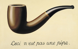
class: center middle main-title section-title-1 # Randomized Trials .class-info[ **Session 5** .light[STA 379/679: Causal Inference <br> Lucy D'Agostino McGowan ] ] --- class: title title-1 center # Potential Outcome <br> <br> .box-1[ What *will* happen to you in the future given you have a particular exposure ] <br> -- .box-inv-1.medium[ **fixed** but **unknown** ] --- class: title title-1 # What do we observe? .box-inv-1.medium[Recall: The causal effect is the comparison of the potential outcomes for the same unit **at the same moment** in time post-exposure] -- .center[  ] --- class: title title-1 # Outcomes for an individual .box-inv-1[ `\(Y_i^{obs}= Y_i(X_i)=\begin{cases}Y_i(0)&\textrm{if }X_i=0\\Y_i(1)&\textrm{if }X_i = 1\end{cases}\)` ] -- <br> .box-1[ `\(Y_i^{mis}= Y_i(1-X_i)=\begin{cases}Y_i(1)&\textrm{if }X_i=0\\Y_i(0)&\textrm{if }X_i = 1\end{cases}\)` ] --- class: section-title-1 title-1 middle # Causal inference is fundamentally a missing data problem .footer[Rubin (1974) Journal of Educational Psychology doi:10.1037/h0037350] --- class: title title-1 ## Stable Unit Treatment Value Assumption .box-inv-1[ The potential outcomes for any unit do not vary with the exposures assigned to other units, and, for each unit, there are no different forms or versions of each exposure level, which lead to different potential outcomes.] .footer[ Imbens and Rubin (2015) *Causal Inference* ] --- class: title title-1 ## Stable Unit Treatment Value Assumption .box-inv-1[ **The potential outcomes for any unit do not vary with the exposures assigned to other units**, and, for each unit, there are no different forms or versions of each exposure level, which lead to different potential outcomes.] .footer[ Imbens and Rubin (2015) *Causal Inference* ] -- .box-1.medium[No Interference] --- class: title title-1 ## Stable Unit Treatment Value Assumption .box-inv-1[ The potential outcomes for any unit do not vary with the exposures assigned to other units, and, for **each unit, there are no different forms or versions of each exposure level, which lead to different potential outcomes.**] .footer[ Imbens and Rubin (2015) *Causal Inference* ] --- class: title title-1 # Exposure assignment .box-inv-1[Understanding the **assignment mechanism** is crucial for understanding the causal effect] -- .box-1[Assignment probability must be **individualistic** (your covariates / potential outcomes can't influence my assignment)] -- .box-1[All units must have **non-zero** probability for all exposures] -- .box-1[Assignment **cannot** depend on the potential outcomes] --- class: title title-1 # Exposure assignment .box-inv-1[Understanding the **assignment mechanism** is crucial for understanding the causal effect] .box-1[Assignment probability must be **individualistic** (your covariates / potential outcomes can't influence my assignment)] .box-2[All units must have **non-zero** probability for all exposures] .box-2[Assignment **cannot** depend on the potential outcomes] --- class: title title-1 # Exposure assignment .box-inv-1[Understanding the **assignment mechanism** is crucial for understanding the causal effect] .box-2[Assignment probability must be **individualistic** (your covariates / potential outcomes can't influence my assignment)] .box-1[All units must have **non-zero** probability for all exposures] .box-2[Assignment **cannot** depend on the potential outcomes] --- class: title title-1 # Exposure assignment .box-inv-1[Understanding the **assignment mechanism** is crucial for understanding the causal effect] .box-2[Assignment probability must be **individualistic** (your covariates / potential outcomes can't influence my assignment)] .box-2[All units must have **non-zero** probability for all exposures] .box-1[Assignment **cannot** depend on the potential outcomes] --- class: title title-1 # Randomized Trials! ```r set.seed(5) d_random <- meeple %>% mutate(x = sample(rep(c(1, 0), each = n / 2)), # coin flip! y_obs = ifelse(x == 1, y1, y0)) ``` --- class: title title-1 # Randomized Trials! ```r d_random %>% summarise(average_noicecream = mean(y0), average_icecream = mean(y1), average_effect = mean(y1 - y0)) ``` ``` ## # A tibble: 1 × 3 ## average_noicecream average_icecream average_effect ## <dbl> <dbl> <dbl> ## 1 1.82 1.82 0 ``` --- class: title title-1 # Randomized Trials! ```r d_random %>% summarise( average_observed = mean(y_obs[x == 1]) - mean(y_obs[x == 0]) ) ``` ``` ## # A tibble: 1 × 1 ## average_observed ## <dbl> ## 1 -0.68 ``` --- class: title-1 title # <svg aria-hidden="true" role="img" viewBox="0 0 448 512" style="height:1em;width:0.88em;vertical-align:-0.125em;margin-left:auto;margin-right:auto;font-size:inherit;fill:currentColor;overflow:visible;position:relative;"><path d="M144 479H48c-26.5 0-48-21.5-48-48V79c0-26.5 21.5-48 48-48h96c26.5 0 48 21.5 48 48v352c0 26.5-21.5 48-48 48zm304-48V79c0-26.5-21.5-48-48-48h-96c-26.5 0-48 21.5-48 48v352c0 26.5 21.5 48 48 48h96c26.5 0 48-21.5 48-48z"/></svg> Pipes .box-1.medium[Where does the name come from?] -- The pipe operator is implemented in the package **magrittr**, it's pronounced "and then". .pull-left[  ] .pull-right[  ] .footer[Adapted from Data Science in a Box] --- class: title title-1 # <svg aria-hidden="true" role="img" viewBox="0 0 448 512" style="height:1em;width:0.88em;vertical-align:-0.125em;margin-left:auto;margin-right:auto;font-size:inherit;fill:currentColor;overflow:visible;position:relative;"><path d="M144 479H48c-26.5 0-48-21.5-48-48V79c0-26.5 21.5-48 48-48h96c26.5 0 48 21.5 48 48v352c0 26.5-21.5 48-48 48zm304-48V79c0-26.5-21.5-48-48-48h-96c-26.5 0-48 21.5-48 48v352c0 26.5 21.5 48 48 48h96c26.5 0 48-21.5 48-48z"/></svg> How does a pipe work? - You can think about the following sequence of actions - find key, unlock car, start car, drive to school, park. - Expressed as a set of nested functions in R pseudocode this would look like: .small[ ```r park(drive(start_car(find("keys")), to = "campus")) ``` ] .footer[Adapted from Data Science in a Box] --- class: title title-1 # <svg aria-hidden="true" role="img" viewBox="0 0 448 512" style="height:1em;width:0.88em;vertical-align:-0.125em;margin-left:auto;margin-right:auto;font-size:inherit;fill:currentColor;overflow:visible;position:relative;"><path d="M144 479H48c-26.5 0-48-21.5-48-48V79c0-26.5 21.5-48 48-48h96c26.5 0 48 21.5 48 48v352c0 26.5-21.5 48-48 48zm304-48V79c0-26.5-21.5-48-48-48h-96c-26.5 0-48 21.5-48 48v352c0 26.5 21.5 48 48 48h96c26.5 0 48-21.5 48-48z"/></svg> How does a pipe work? .small[ ```r park(drive(start_car(find("keys")), to = "campus")) ``` ] - Writing it out using pipes give it a more natural (and easier to read) structure: .small[ ```r find("keys") %>% start_car() %>% drive(to = "campus") %>% park() ``` ] .footer[Adapted from Data Science in a Box] --- class: title title-1 # <svg aria-hidden="true" role="img" viewBox="0 0 448 512" style="height:1em;width:0.88em;vertical-align:-0.125em;margin-left:auto;margin-right:auto;font-size:inherit;fill:currentColor;overflow:visible;position:relative;"><path d="M144 479H48c-26.5 0-48-21.5-48-48V79c0-26.5 21.5-48 48-48h96c26.5 0 48 21.5 48 48v352c0 26.5-21.5 48-48 48zm304-48V79c0-26.5-21.5-48-48-48h-96c-26.5 0-48 21.5-48 48v352c0 26.5 21.5 48 48 48h96c26.5 0 48-21.5 48-48z"/></svg> What about other arguments? To send results to a function argument other than first one or to use the previous result for multiple arguments, use `.` ```r starwars %>% filter(species == "Human") %>% lm(mass ~ height, data = .) ``` .footer[Adapted from Data Science in a Box] --- class: title title-1 # Randomized trial * The easiest way to establish a causal effect is to run a controlled trial! -- * Even very controlled experiments often have things that make them tricky to interpret: people drop out, non-compliance with treatment, interference --- class: title title-1 # Randomized trial .box-2[Assignment probability must be **individualistic** (your covariates / potential outcomes can't influence my assignment)] .box-1[All units must have **non-zero** probability for all exposures] .box-2[Assignment **cannot** depend on the potential outcomes] --- class: title title-1 # Randomized trial .box-1[Assignment probability must be **individualistic** (your covariates / potential outcomes can't influence my assignment)] .box-2[All units must have **non-zero** probability for all exposures] .box-1[Assignment **cannot** depend on the potential outcomes] --- class: title title-1 # Notation .box-inv-1.medium[ .huge[ `\(\mathbf{Y}(0), \mathbf{Y}(1)\)` ] ] -- <br> .box-1[ vectors of potential outcomes where the `\(i\)`th is equal to `\(Y_i(0)\)` / `\(Y_i(1)\)` ] --- class: title title-1 # Notation .box-inv-1.medium[ .huge[ `\(\mathbf{X}\)` ] ] -- .box-1[ vector of exposure assignment ] --- class: section-title-1 title-1 middle # Causal inference is fundamentally a missing data problem .footer[Rubin (1974) Journal of Educational Psychology doi:10.1037/h0037350] --- class: title title-1 # Outcomes for an individual .box-inv-1[ `\(Y_i^{obs}= Y_i(X_i)=\begin{cases}Y_i(0)&\textrm{if }X_i=0\\Y_i(1)&\textrm{if }X_i = 1\end{cases}\)` ] -- <br> .box-1[ `\(Y_i^{mis}= Y_i(1-X_i)=\begin{cases}Y_i(1)&\textrm{if }X_i=0\\Y_i(0)&\textrm{if }X_i = 1\end{cases}\)` ] --- class: title title-1 # Outcomes for an individual .box-inv-1[ `\(Y_i(0)= \begin{cases}Y_i^{mis}&\textrm{if }X_i=1\\Y_i^{obs}&\textrm{if }X_i = 0\end{cases}\)` ] <br> -- .box-1[ `\(Y_i(1)= \begin{cases}Y_i^{mis}&\textrm{if }X_i=0\\Y_i^{obs}&\textrm{if }X_i = 1\end{cases}\)` ] --- class: section-title-1 title-1 middle # Causal inference is fundamentally a missing data problem .footer[Rubin (1974) Journal of Educational Psychology doi:10.1037/h0037350] -- .box-inv-1[If we impute the missing outcomes, we can know the value of any causal estimand] --- class: title-1 title # Average treatment effect estimand <br> .box-inv-1[ `$$\tau=\frac{1}{N}\sum_{i=1}^N(Y_i(1)-Y_i(0))=\bar{Y}(1)-\bar{Y}(0)$$` ] --- class: title-1 title # Average treatment effect estimand <br> .box-inv-1[ `$$\bar{Y}(0)=\frac{1}{N}\sum_{i=1}^NY_i(0)\textrm{ and }\bar{Y}(1) = \frac{1}{N}\sum_{i=1}^NY_i(1)$$` ] --- class: title title-1 # Randomized experiment .box-1[ `$$N_{e} = \sum_{i=1}^NX_i$$` are assigned to the exposure ] --- class: title title-1 # Randomized experiment .box-1[ `$$N_c = \sum_{i=1}^N(1-X_i)$$` are assigned to the control group ] --- class: title title-1 # Estimator for average treatment effect <br> .box-inv-1[ .huge[ `$$\hat{\tau}=\bar{Y}_e^{obs}-\bar{Y}_c^{obs}$$` ] ] --- class: center <figure> <img src = "img/estimand.jpeg" width = "50%"></img> </figure> .footer[ Simon Grund on [Twitter](https://twitter.com/simongrund89/status/1085929122860359680?lang=bg) ] --- class: title-1 title # Average treatment effect estimand <br> .box-inv-1[ `$$\tau=\frac{1}{N}\sum_{i=1}^N(Y_i(1)-Y_i(0))=\bar{Y}(1)-\bar{Y}(0)$$` ] --- class: title title-1 # Estimator for average treatment effect <br> .box-inv-1[ .huge[ `$$\hat{\tau}=\bar{Y}_e^{obs}-\bar{Y}_c^{obs}$$` ] ] --- class: title title-1 # Estimator for average treatment effect <br> .box-inv-1[ .huge[ `$$\bar{Y}_c^{obs}=\frac{1}{N_c}\sum_{i:X_i=0}Y_i^{obs}$$` ] ] --- class: title title-1 # Estimator for average treatment effect <br> .box-inv-1[ .huge[ `$$\bar{Y}_e^{obs}=\frac{1}{N_e}\sum_{i:X_i=1}Y_i^{obs}$$` ] ] --- class: title title-1 # Estimator for average treatment effect ```r d_random %>% summarise( average_observed = mean(y_obs[x == 1]) - mean(y_obs[x == 0] ) ) ``` ``` ## # A tibble: 1 × 1 ## average_observed ## <dbl> ## 1 -0.68 ``` --- class: title title-1 # Estimator for average treatment effect .box-1.medium[Why does this work?] -- .box-inv-1.medium[We know:] -- .box-1[ `\(Y_i^{obs}=Y_i(1)\)` if `\(X_i=1\)` ] -- .box-1[ `\(Y_i^{obs}=Y_i(0)\)` if `\(X_i=0\)` ] --- class: title title-1 # We can rewrite the estimator <br> .box-inv-1[ `$$\hat\tau=\frac{1}{N}\sum_{i=1}^N\left(\frac{X_iY_i(1)}{N_e/N}-\frac{(1-X_i)Y_i(0)}{N_c/N}\right)$$` ] --- class: title title-1 # We can rewrite the estimator .box-inv-1[ `$$\frac{1}{N_e}\sum_{i:X_i=1}Y_i^{obs}-\frac{1}{N_c}\sum_{i:X_i=0}Y_i^{obs}$$` ] --- class: title title-1 # We can rewrite the estimator .box-inv-1[ `$$\frac{1}{N_e}\sum_{i:X_i=1}\color{purple}{Y_i^{obs}}-\frac{1}{N_c}\sum_{i:X_i=0}Y_i^{obs}$$` ] --- class: title title-1 # We can rewrite the estimator .box-inv-1[ `$$\frac{1}{N_e}\sum_{i:X_i=1}\color{purple}{Y_i(1)X_i}-\frac{1}{N_c}\sum_{i:X_i=0}Y_i^{obs}$$` ] --- class: title title-1 # We can rewrite the estimator .box-inv-1[ `$$\frac{1}{N_e}\sum_{i:X_i=1}{Y_i(1)X_i} -\frac{1}{N_c}\sum_{i:X_i=0}\color{purple}{Y_i^{obs}}$$` ] --- class: title title-1 # We can rewrite the estimator .box-inv-1[ `$$\frac{1}{N_e}\sum_{i:X_i=1}{Y_i(1)X_i} -\frac{1}{N_c}\sum_{i:X_i=0}\color{purple}{Y_i(0)(1-X_i)}$$` ] --- class: title title-1 # We can rewrite the estimator .box-inv-1[ `$$\sum_{i:X_i=1}\frac{Y_i(1)X_i}{\color{purple}{N_e} }-\sum_{i:X_i=0}\frac{Y_i(0)(1-X_i)}{\color{purple}{N_c}}$$` ] --- class: title title-1 # We can rewrite the estimator .box-inv-1[ `$$\color{purple}{\frac{1}{N}}\left(\sum_{i:X_i=1}\frac{Y_i(1)X_i}{N_e/\color{purple}{N} }-\sum_{i:X_i=0}\frac{Y_i(0)(1-X_i)}{N_c/\color{purple}{N}}\right)$$` ] --- class: title title-1 # We can rewrite the estimator .box-inv-1[ `$$\frac{1}{N}\color{purple}{\sum_{i=1}^N}\left(\frac{Y_i(1)X_i}{N_e/{N} }-\frac{Y_i(0)(1-X_i)}{N_c/{N}}\right)$$` ] --- class: title title-1 # What is random? .box-inv-1[ `$$\frac{1}{N}\sum_{i=1}^N\left(\frac{Y_i(1)X_i}{N_e/N }-\frac{Y_i(0)(1-X_i)}{N_c/N}\right)$$` ] --- class: title title-1 # What is random? .box-inv-1[ `$$\frac{1}{N}{\sum_{i=1}^N}\left(\frac{Y_i(1)\color{purple}{X_i}}{N_e/N}-\frac{Y_i(0)(1-\color{purple}{X_i})}{N_c/N}\right)$$` ] --- class: title title-1 # Randomized experiment <br> .box-inv-1[ `$$P_X(X_i = 1 | \mathbf{Y}(0), \mathbf{Y}(1)) = \mathbb{E}_X[X_i|Y(0), Y(1)] = N_e/N$$` ] --- class: title title-1 # Randomized experiment <br> .box-inv-1[ `$$P_X(X_i = 0 | \mathbf{Y}(0), \mathbf{Y}(1)) = \\\mathbb{E}_X[1 - X_i|Y(0), Y(1)] = N_c/N$$` ] --- class: title title-1 # Randomized exeriment: unbiased .box-inv-1[ `$$\mathbb{E}_X[\hat\tau|\mathbf{Y}(0),\mathbf{Y}(1)]=\\\frac{1}{N}\sum_{i=1}^N\left(\frac{\mathbb{E}_X[X_i]Y_i(1)}{N_e/N}-\frac{\mathbb{E}_X[1-X_i]Y_i(0)}{N_c/N}\right)$$` ] --- class: title title-1 # Randomized exeriment: unbiased .box-inv-1[ `$$\mathbb{E}_X[\hat\tau|\mathbf{Y}(0),\mathbf{Y}(1)]=\\\frac{1}{N}\sum_{i=1}^N\left(\frac{(N_e/N)Y_i(1)}{N_e/N}-\frac{(N_c/N)Y_i(0)}{N_c/N}\right)$$` ] --- class: title title-1 # Randomized exeriment: unbiased .box-inv-1[ `$$\mathbb{E}_X[\hat\tau|\mathbf{Y}(0),\mathbf{Y}(1)]=\\\frac{1}{N}\sum_{i=1}^N\left(Y_i(1)-Y_i(0)\right)=\tau$$` ] --- class: title title-1, center # <svg aria-hidden="true" role="img" viewBox="0 0 640 512" style="height:1em;width:1.25em;vertical-align:-0.125em;margin-left:auto;margin-right:auto;font-size:inherit;fill:currentColor;overflow:visible;position:relative;"><path d="M624 416H381.54c-.74 19.81-14.71 32-32.74 32H288c-18.69 0-33.02-17.47-32.77-32H16c-8.8 0-16 7.2-16 16v16c0 35.2 28.8 64 64 64h512c35.2 0 64-28.8 64-64v-16c0-8.8-7.2-16-16-16zM576 48c0-26.4-21.6-48-48-48H112C85.6 0 64 21.6 64 48v336h512V48zm-64 272H128V64h384v256z"/></svg> Application Exercise <br><br> .huge[[github.com/sta-679-s22](https://github.com/sta-679-s22)] ---